AgroScan Report
Soils represent the largest terrestrial carbon pool globally and play a critical role as carbon sinks through soil carbon sequestration, where atmospheric CO₂ is stored as soil organic matter (Paustian et al., 2019)[1]. Agricultural soils with high soil organic carbon (SOC) content deliver significant environmental and agronomic co- benefits: improved long-term productivity, increased biodiversity, and preservation of ecosystem services (European Commission, 2021)[2]. Consequently, monitoring and enhancing SOC stocks has become a priority within major policy frameworks, including the EU Soil Strategy for 2030 that translates into the EU Soil Monitoring Law (European Commission, 2021[2]; European Parliament, 2025)[3].
Despite this recognized importance, farmers face substantial barriers when integrating SOC monitoring into their agricultural practices. Conventional soil sampling requires repeated field and laboratory work across extended time periods, creating significant cost, labor, and scalability constraints that limit its routine application in large agricultural areas (Ihasusta et al., 2026)[4].
Machine learning-based remote sensing models have emerged as a promising approach to address these limitations (Nguyen et al., 2022[15]; Yuzugullu et al., 2024[21]). By leveraging satellite-derived data, these models offer scalable and cost-efficient SOC estimation and allow a baseline to be established using historic satellite imagery to assess the impact of sustainable soil management (SSM) practices over time. Existing SOC prediction tools, however, only provide limited transparency regarding their underlying methodology. Many commercial SOC monitoring platforms are designed for carbon credit generation, compliance, and monetization based on SOC changes on field- or farm-level. This use case provides an accounting system but places less emphasis on model transparency and development of agronomic understanding of the user. As a result, users are constrained in their ability to critically evaluate model outputs, infer drivers of soil evolution patterns, and make adaptive field management decisions.
This motivated the central research question of the present study:
How can visual analytics empower farmers to monitor and manage soil carbon stocks in agricultural soils over the long term?
AgroScan addresses this question by providing a novel open-source platform utilizing visual analytics principles as a means of increasing the transparency and interpretability of the model to empower the farmer in their decision-making. Overall, its main contributions are: (1) User requirements derived in initial exploratory interviews, and then confirmed in a final evaluation; (2) ML model prototype for SOC prediction from satellite data; (3) Visual analytics design enabling interpretability of model outputs for decision support; (4) End-to-end integration of model and interface into an open-source deployed platform.
The use of remote sensing combined with machine learning for SOC prediction in agricultural soils has become more established in academic research. Nguyen et al. (2022)[15] demonstrated a multi-sensor data fusion model combining multispectral image data from Sentinel-2 and synthetic aperture radar data from Sentinel-1, achieving high prediction accuracy (R² = 0.870, RMSE = 1.818 t/ha). The study highlighted that incorporating derived predictor features — including vegetation and soil indices calculated from raw band values — significantly improved model performance.
Complementing this, Guo et al. (2021)[5] showed that Sentinel-2 optical data and crop- growth indices are particularly effective predictors for agricultural soils, which typically exhibit lower topological variability than other land use types. Similar results supporting the use of remote sensing for carbon prediction were demonstrated by Yuzugullu et.al. (2024)[21], Beisekenov et.al. (2025)[22], Zhang et.al. (2019)[23]. Taken together, these studies confirm that the technical foundation for remote sensing-based SOC prediction in agricultural contexts is well established.
Based on the academic foundation, several commercial platforms for remote-sensing-based carbon monitoring exist, highlighting the demand for such solutions such as Smart Cloud Farming (Smart Cloud Farming, n.d.)[25], Spacenus (Spacenus, n.d.)[26], Soyle (Soyle, n.d.)[27], Agreena (Agreena, n.d.)[28], and Farmonaut (Farmonaut, n.d.)[9]. Common applications include soil sampling location algorithms, variable-rate fertilization, yield productivity monitoring, and measurement, reporting, and verification (MRV) for carbon credit schemes, enabling farmers to optimize inputs and generate additional income. In contrast, AgroScan targets long-term decision support by providing insights into the effects of crop rotations on soil organic carbon (SOC) and humus levels, a use case for which no dedicated commercial solution was identified. This empowers the farmer to make long-term sustainable decisions. Through visualizations of the temporal evolution of SOC and derived soil organic matter (SOM) content based on the van Bemmelen factor, AgroScan facilitates the identification of long-term trends related to the crop rotation and farming practices. Furthermore, whereas many existing tools lack transparency regarding their underlying models, AgroScan provides methodological explanations tailored to non-technical users, detailed reports, and visualization and communication of prediction uncertainty.
Several visual analytics applications have investigated the use of interactive visualizations to support long-term agricultural decision-making. These systems generally aim to enable users to explore temporal developments in agricultural and environmental indicators while relating them to spatial patterns and management interventions. GeoVisage, a web-based agricultural decision support platform co-developed by Nipissing University and agricultural producers in Ontario, Canada, integrated horizon charts and small-multiple visualizations to facilitate the exploration of spatiotemporal datasets (Wachowiak et al., 2017)[29]. Similarly, Htun et al. proposed a dashboard for identifying water stress and irrigation requirements by combining map-based visualizations with temporal line charts. Their user evaluation, however, revealed high mental demand and effort, highlighting the importance of intuitive workflows and guided analytical processes in agricultural visual analytics systems (Htun et al., 2022)[30]. Dhaliwal et al. also demonstrated the applicability of line charts for analysing agricultural time-series data, although their implementation lacked a coordinated dashboard environment (Dhaliwal et al., 2023)[31]. Collectively, these studies indicate the potential of integrating spatial and temporal visualizations for analysing long-term agricultural developments, while also underscoring the need for cohesive interfaces that minimise cognitive load and effectively guide users through exploratory analyses.
AgroScan's target users are farmers who use software-based farm management tools, and are interested in carbon farming and sustainable soil management (SSM) practices. To identify user requirements, we conducted exploratory interviews with two farmers in the municipality Eichstätt in Bavaria, Germany. The idea of an interactive remote-sensing SOC prediction tool was derived from literature research and pitched to the farmers to understand its relevance in their work. Subsequently, questions about the tool were asked to identify key user requirements.
- J. (28), raised on an organic farm with crops and cattle, combines practical farming experience with his current work in agricultural policy as a civil servant in the Bavarian department of agriculture.
- A. (54), is a full-time certified organic farmer managing 145 ha of arable land. He is a professionally trained farmer with formal agricultural education and specializes in organic farming.
A typical use case of a farmer for the AgroScan tool is the routine monitoring of SOC content of their agricultural fields to identify long-term trends in SOC and derived SOM level of their fields in dependence on crop rotation and other targeted SSM practices.
Based on the interviews the following user requirements were defined to inform the website design:
- Explainable decision support
- The interface guides user through the SOC analysis process while requiring minimal technical expertise and highlighting important information like model limitations
- SOC predictions are presented together with contextual information like crop rotations, required for interpretation
- The interface supports perceptual inference by allowing users to visually associate changes in SOC with crop rotations and management measures
- Integrated field data management dashboard
- The dashboard summarizes and displays all relevant information in a comprehensive and clear manner, both at the field and farm levels.
- The dashboard functionalities support the identification and assessment of long-term trends in dependence on crop rotation and other SSM practices.
- Transparent model-user interaction
- The tool adequately informs about the underlying data, methodology and limitations of the model, regardless of the technological expertise of the user.
- The tool provides several options of interacting with and developing the underlying model, accommodating different levels of technical expertise.
1. Selection of case region
Germany was selected as the case region due to its significant agricultural sector,
strong policy relevance, and high soil data availability. Around half of Germany’s land
area is used for agriculture, making it one of the European Union’s largest agricultural
producers (Federal Ministry of Food and Agriculture [BMEL], 2023)[11]. In addition,
Germany must comply with the European Union Soil Monitoring Law by 2028,
increasing the demand for scalable and cost-effective soil monitoring methods
(European Union, 2025)[12]. AgroScan could support these future monitoring requirements
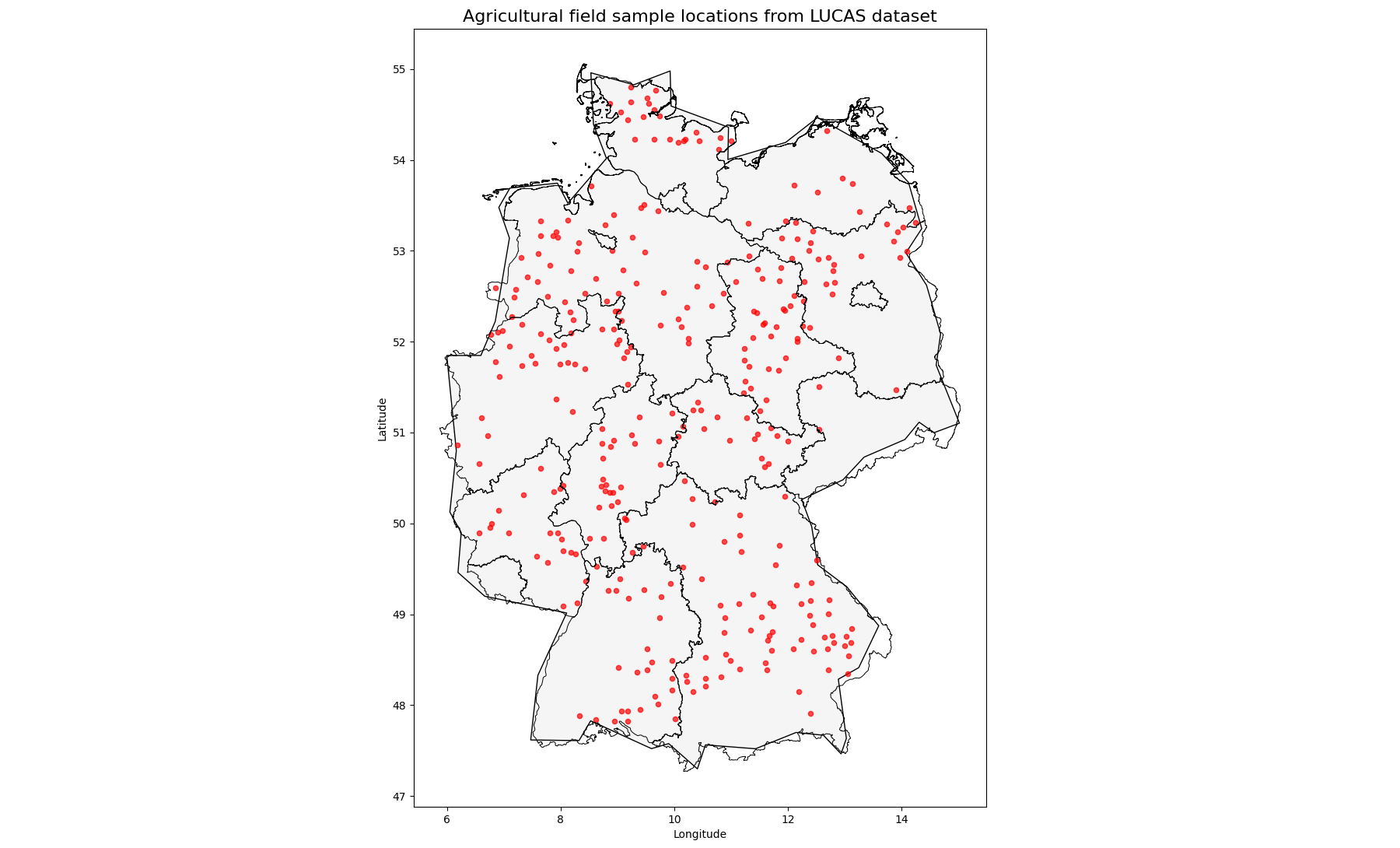
through large-scale SOC assessments. Germany also offers strong data availability:
The LUCAS 2019 soil dataset has 332 agricultural sampling locations in Germany, of
which 270 could be matched to Sentinel-2 data (Fernández-Ugalde et.al., 2022)[24]; Fig. 1).
2. Data sources
Two publicly available and freely accessible datasets were selected as the foundation
for the AgroScan model to support the project’s commitment to reproducibility and low
barriers to adoption.
Input data: Sentinel-2 multispectral imagery was selected as the primary input data source. It is operated by the European Space Agency as part of the Copernicus program and provides near-global coverage with a site revisit frequency of five days. This ensures a high availability of observations. It is freely accessible via the Copernicus API. Its 13 spectral bands span the Visible, Near-Infrared (NIR), and Short-Wave Infrared (SWIR) regions of the electromagnetic spectrum (Copernicus Sentinel, n.d.)[13] Level-2A products were used, which provide atmospherically corrected Bottom-of-Atmosphere reflectance values. This improves the physical interpretability and comparability of the data.
From the full set of available bands, 10 were selected as model inputs: B2, B3, B4, B5, B6, B7, B8, B8A, B11, and B12. These bands cover critical spectral regions and enable inference of key biophysical properties relevant to SOC estimation, including vegetation condition, soil moisture, and crop growth status (Ngyuen et al., 2022)[15].
Target variable: The LUCAS Topsoil dataset was selected as the source of ground-truth SOC measurements. It is coordinated by Eurostat and the European Commission’s Joint Research Centre and provides georeferenced soil samples collected across EU Member States from the topsoil layer (0–20 cm), which is most relevant for SOC dynamics in agricultural systems (European Commission, JRC, 2021)[16]. The dataset includes land-use classification, enabling filtering to cropland samples only. This ensures consistency between the target variable and the modelling domain. Its EU- wide, harmonized design makes it well-suited as ground truth for remote sensing– based SOC prediction. The upcoming LUCAS 2022 Topsoil release will enable future model retraining with more recent observations.
3. Data collection and processing
The data collection and processing pipeline is based on a GitHub repository of the
Computer Vision for Intelligent Mobility System Laboratory of the Technische
Hochschule Ingolstadt (CVIMS, 2025)[17]. We updated the pipeline to the current
Copernicus OData communication protocol, added a feature transformation, and
modified it to be compatible with our interactive use case. Building on the existing
CVIMS framework (2025)[17], the following outlines our team’s main contributions.
Feature transformation: Building on the selected raw band values, 13 additional predictor features were derived: 7 vegetation indices, 4 soil indices, and 2 cyclical temporal features encoding the month of observation. This feature engineering step follows Nguyen et al. (2022)[15], who demonstrated that derived indices correlate more strongly with agricultural SOC than raw spectral bands alone, with the Soil-Adjusted Vegetation Index (SAVI) identified as the single most important predictor. The inclusion of crop-growth indices is particularly appropriate for agricultural soils, which exhibit comparatively low topological variability, making spectral signals related to vegetation and soil surface conditions the dominant source of predictive information (Guo et al., 2021)[5].
The two temporal features encode the survey month as sine and cosine components allowing the model to capture seasonal variation in surface reflectance while avoiding artificial discontinuities between December and January.
Overview of predictor features
| Predictor feature | Acronyms | Formulas |
|---|---|---|
| Ratio Vegetation Index | RVI | NIR / Red |
| Normalized Difference Vegetation Index | NDVI | (NIR − Red) / (NIR + Red) |
| Green Normalized Difference Vegetation Index | GNDVI | (NIR − Green) / (NIR + Green) |
| Normalized Difference Index using Bands 4 & 5 of S-2 | NDI45 | (RE1 − Red) / (RE1 + Red) |
| Soil Adjusted Vegetation Index | SAVI | (1 + L) × (NIR − Red) / (L + NIR + Red), L = 0.5 |
| Inverted Red-Edge Chlorophyll Index | IRECI | (NIR − Red) / (RE1 / RE2) |
| Modified Chlorophyll Absorption in Reflectance Index | MCARI | [(RE1 − Red) − 0.2 × (RE1 − Green)] × (RE1 / NIR) |
| Brightness index | BI | √((Red² + Green²) / 2) |
| Brightness index 2 | BI2 | √((Red² + Green² + NIR²) / 3) |
| Redness index | RI | Red² / Green² |
| Color index | CI | (Red − Green) / (Red + Green) |
| Month (sin) | sin_month | sin(2π·month/12) |
| Month (cos) | cos_month | cos(2π·month/12) |
Note: Band wavelengths of S-2: B2 = Blue (492 nm), B3 = Green (560 nm), B4 = Red (665 nm), B5 = Red-edge 1 (RE1) (704 nm), B6 = Red-edge 2 (RE2) (740 nm), B7 = Red-edge 3 (RE3) (783 nm), B8 = Near-infrared (NIR) (833 nm), B8A = Narrow-NIR (865 nm), B11 = SWIR1 (1614 nm), B12 = SWIR2 (2202 nm). (Adapted from Ngyuen et.al., 2022)[15]
Interactive use case: A fixed reference min-max normalization was implemented for both Sentinel-2 band values and all derived indices. Unlike dataset-dependent normalization, which scales values relative to the minimum and maximum of whichever dataset is being processed, the fixed approach computes reference minimum and maximum values once from a representative dataset — here, the full German training set — and applies those constants consistently at every subsequent stage of the pipeline.
This design decision was motivated to fit the interactive use case of AgroScan. At inference time, a farmer submits the GPS coordinates of their field, triggering the download of a small, location-specific Sentinel-2 datafile. A dataset-dependent normalization applied to this single observation would produce meaningless scaled values. The fixed reference approach ensures that the normalization applied to the farmer’s input is identical to that used during training, preserving the statistical relationship between features that the model learned. This makes the pipeline fully reusable from training to individual farmer queries without modification. Values outside the reference range are clipped to the unit interval to handle edge cases.
Normalization logic
The fixed reference minimum and maximum values are computed once from a representative dataset using the python scripts calculate_band_ranges.py and calculate_index_ranges.py and saved to a respective .json file. For the normalization each raw value \(x\) is transformed to
\[x'=\frac{x-x_{\min}}{x_{\max}-x_{\min}}\]
and then, if needed, clipped to the unit interval: \(x' \leftarrow \min(1,\max(0,x'))\). If \(x_{\max}=x_{\min}\) the implementation returns 0 to avoid division by zero and NaN/inf values are replaced with 0 afterwards.
1. Selection of model
The model architecture and implementation used in this work are based on the
approach presented by Kammerlander (2025)[14]. Kammerlander evaluated three machine
learning approaches for predicting soil nutrient levels across Europe: XGBoost,
Random Forest, and Fully Connected Neural Networks (FCNNs). Model performance
was assessed using Root Mean Squared Error (RMSE) for several soil properties,
including phosphorus, nitrogen, potassium, and pH.
The results showed that the FCNN architecture achieved the best overall performance. While XGBoost and Random Forest produced similar results for pH estimation, FCNN outperformed the other methods for nutrients with high variability.
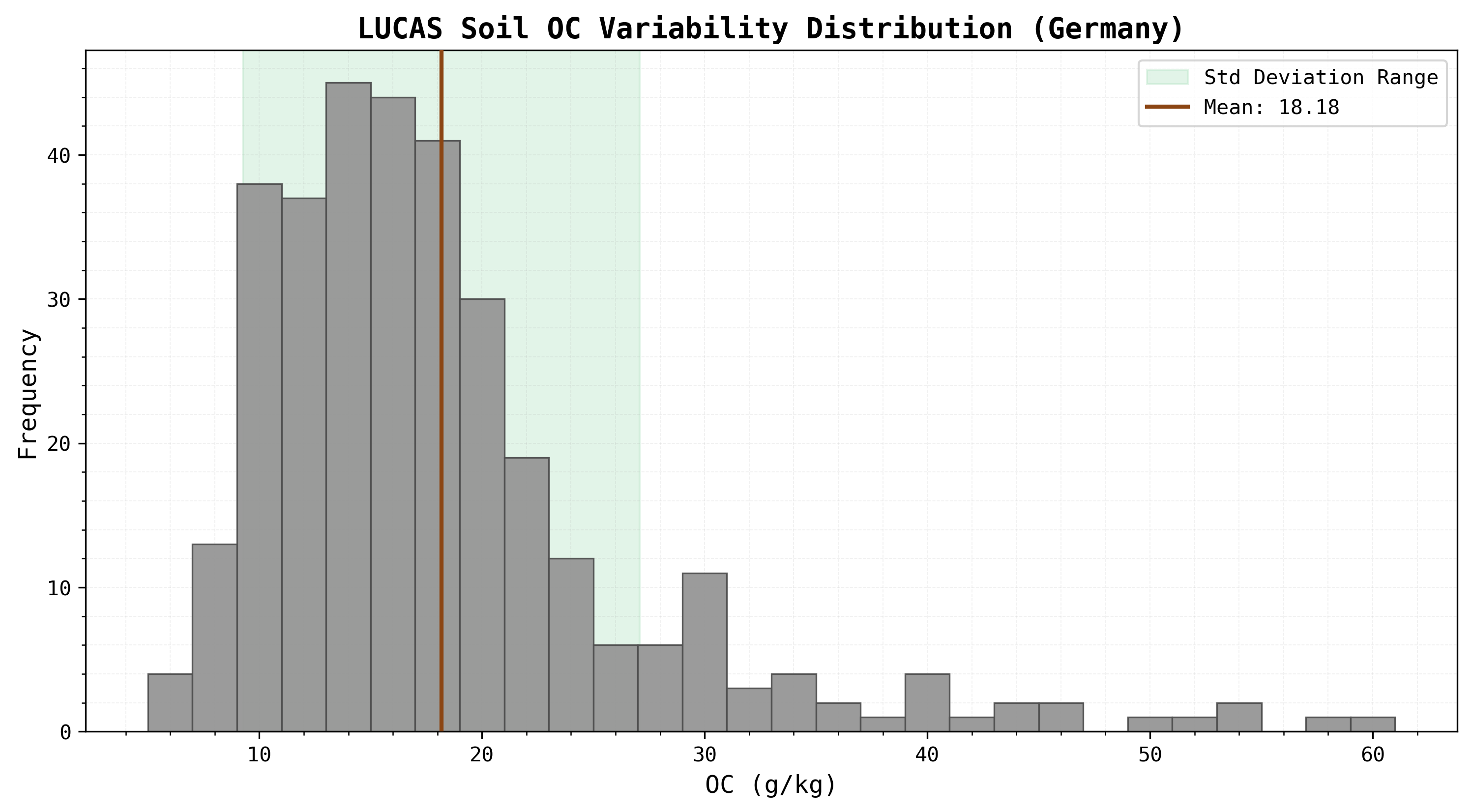
Within the LUCAS dataset filtered for German croplands, organic carbon (OC) has a mean value of 18.18 g/kg and a standard deviation of ±8.91 g/kg, indicating substantial variability across samples. This behavior is comparable to the nutrient variables analyzed by Kammerlander (2025)[14], where high variability strongly influenced model performance. Since FCNNs are well suited for learning nonlinear relationships and modelling heterogeneous nutrient distributions, they are considered the most appropriate architecture for this prediction task.
What is a FCNN
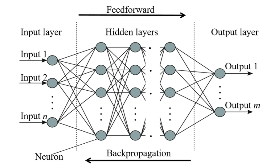
FCNNs, also referred to as multilayer perceptron, are feedforward artificial neural networks in which each neuron of one layer is connected to all neurons of the subsequent layer. FCNNs are trained using the backpropagation algorithm introduced by Rumelhart (1986)[19]. Through multiple hidden layers and nonlinear activation functions, FCNNs are capable of learning complex nonlinear relationships between input features and target variables.
The ML model behind AgroScan
Model architecture
The network is constructed dynamically as a sequence of linear layers with ReLU
activation and dropout after each hidden layer, followed by a single linear output
neuron for predicting OC. Model training is performed with backpropagation in PyTorch
using mini-batches and RMSE as optimization objective. Weight decay of 0.01 is
applied for regularization.
Hyperparameter tuning
Hyperparameter tuning is performed using Optuna. In each trial, the following
hyperparameters are sampled:
- Number of hidden layers: 3 to 9 layers
- Number of Neurons per Layer: 8 to 128 (step size 4)
- Dropout Rate: continuous between 0.1 and 0.5
- Learning Rate: 0.0001 to 0.01 (log scale)
- Optimizer: SGD or Adam
- Batch Size: 16, 32, or 64
Model training
For every trial, a new FCNN architecture is built from the sampled layer widths and
dropout rates, trained for 20 epochs, and evaluated on the held-out test set. The
currently best model (lowest test RMSE so far) is saved to disk as a checkpoint file
(.pth), together with architecture metadata (input size, hidden sizes, dropout rates,
output size, and loss type).
For FCNN training, the dataset is split once into train and test subsets using an 80/20
ratio. Thus, FCNN validation is a single random holdout split.
Model employment
The prediction is implemented in run_pipeline_from_gps.py. The same feature-
processing logic used during training is reused to prepare the dataset. Sentinel-2
imagery for each location is downloaded, after which the pixel values around the
sampled point are extracted, the spectral bands are normalized, and the derived
features are computed. The transformed dataset is then passed to the neural network,
which outputs the predicted carbon content value, stored as OC in the repository.
Using the described model architecture, a RMSE of 6.536 OC g/kg was obtained. This is relatively high, primarily due to the limited dataset size due to computational constraints within the scope of this project. The primary focus of the project was the integration of the machine learning model into a deployable pipeline and interactive web-based platform to make the information accessible to farmers.
2. Model interaction
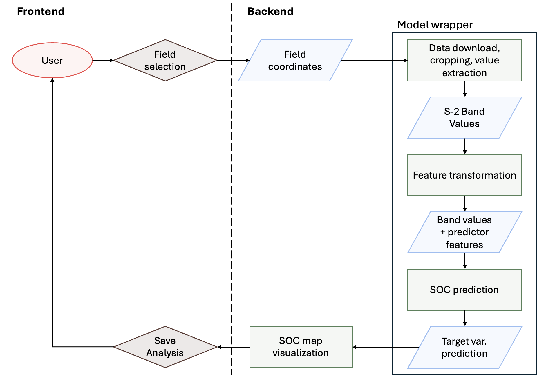
The data collection, processing and model prediction pipeline was compiled into a
wrapper script (run_pipeline_from_gps.py) and placed into the website backend. It uses
the same workflow as during model training (see Fig. 3). The wrapper
enables the user to interact with the model: They select their field, from there the field
coordinates are extracted in a grid system and used as input for the model wrapper. As
output, it provides a visualization for the user of the prediction in the form of a map,
and detailed information in the personal dashboard making the SOC information
easy-to-access for the farmer.
To speed up processing, the system reuses previously downloaded Sentinel scenes and cropped outputs whenever possible. Raw Sentinel scenes are cached as raw data, while cropped per-point outputs are stored together with metadata. The backend generates a fixed 60×60 m grid over the selected field polygon and uses the grid centers as analysis points. To maximize cache reuse, the grid is dynamically aligned to existing cached points by selecting the anchor position with the highest overlap. If a cached point is found within a 10 m radius, the existing cropped image is reused instead of generating a new one. As a result, only when no data is available, missing scenes are downloaded and cropped significantly reducing processing time.
This same mechanism can be extended to a background sync process that proactively downloads and updates cached scenes for a farm/region when new Sentinel acquisitions arrive, enabling near-instant analysis for farmers without waiting for on- demand downloads.
The user requirements are addressed through the following design solutions: a simple step-by-step analysis workflow, an analytical personal dashboard, and full methodological transparency through open-source code, public data sources, and accessible documentation.
Interaction Workflow
Analysis Core User Workflow: The core user workflow follows a step-by-step navigation
model illustrated as a green arrow in Fig. 4. Several interaction design principles were applied
to maximize usability and reduce cognitive load. Pattern affordance is established by consistently
coloring every workflow-advancing button in AgroScan's signature green, which helps users easily
orient themselves. To prevent misguidance, these action buttons remain greyed out until they become
active in the sequence. Established icons and interface conventions, e.g., a magnifier for location
search, build on familiarity with widely used services such as Google Maps. Additionally, several
features for error prevention were implemented: a pop-up summarizing the main limitations in the
application of the model, and if a user tries to start the analysis without a field selected,
another pop-up message guides them to the field selection. To reduce memory requirements and support
first-time users, instructions guide the user in each step in the analysis page, with only the
current step visible.
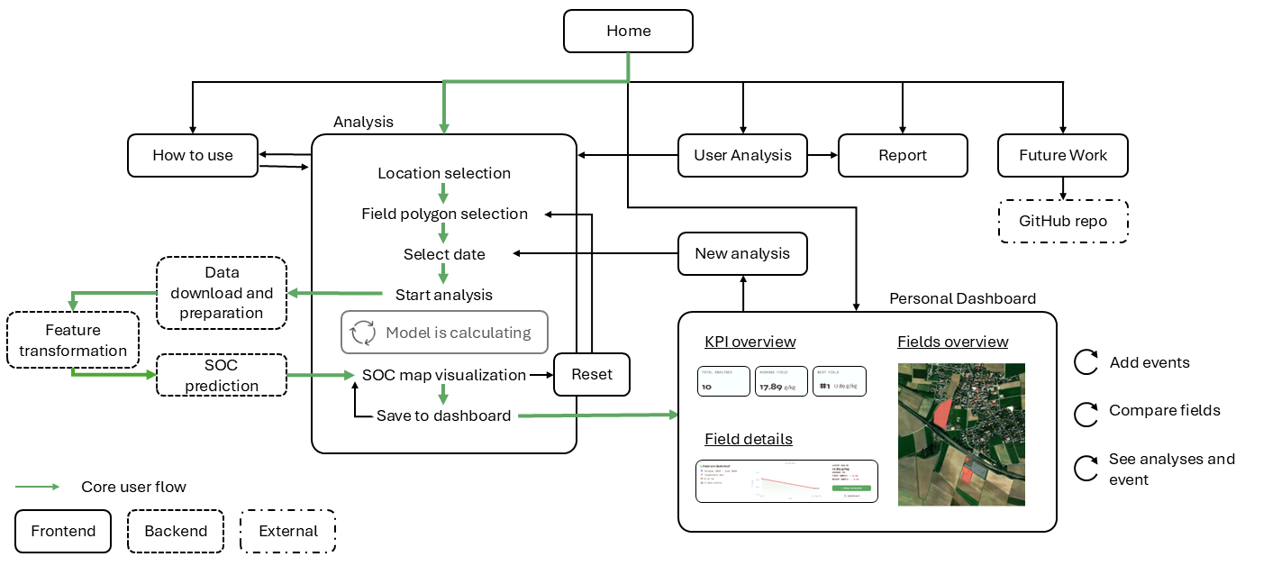
Personal Dashboard: The personal analytical dashboard follows Shneiderman's Visual Information Seeking Mantra (Shneiderman, 1996)[32] by employing a card-based, hierarchical information architecture. An overview map visualizes all fields analyzed by the farmer. Additionally, a KPI strip provides a high-level aggregation of field information (total fields, analyses, etc.). Below, each field is presented as a content card in a card-based layout, allowing for easy scalable information content. Each content card includes embedded field metadata, a micro-visualization of OC content over time, and inline numeric annotations to increase ease-of-use. Several UX interaction patterns were integrated. The farmer has the option to refine the visible selection via the sort, filter, and comparison functions. Additional field-level analyses details can be accessed via the “Click to see all analyses and events” button, alongside a dedicated button to initiate a new analysis for the same field to support long-term SOC monitoring. To support the farmer in identifying the impact of their crop rotation on the SOC level, the planted crop can be added as an event to the line chart of OC over time. Additionally, the SOC value is converted to the more familiar SOM value via the van Bemmelen factor (FAO, n.d.)[34]. Combined with contextualizing reference information such as SOC variation within the field, and numerical historical changes, the farmer can develop an agronomic understanding of the impact of their crop rotation and derive adaptive field management decisions.
Information Design
Spatial predictions of soil organic carbon (SOC) are communicated through an interactive map that
highlights intra-field variability. This allows the identification of low-SOC zones and support
targeted interventions. Predicted SOC values are represented using the color-blind-friendly Plasma
color palette (Garnier et al., 2024)[33], which is applied consistently throughout the map
visualizations to ensure visual coherence. The corresponding color classes are derived from the
SOC value distribution of the LUCAS soil dataset and are explained via a legend. Grounding the
classification in a well-established reference dataset increases the transparency and interpretability
of the displayed results.
In addition to the spatial representation that functions as an overview, temporal developments in SOC are visualized using a line chart. The chart is complemented by contextual information, such as crop rotation practices, enabling users to relate changes in predicted SOC levels to management decisions and to identify long-term trends. Presenting multiple coordinated views facilitates the interpretation of both spatial and temporal patterns and supports informed decision-making. Prediction uncertainty is represented by a fading effect as a conceptual placeholder. Meaningful uncertainty estimates cannot currently be derived due to the prototype nature of the ML model but could be incorporated in future iterations through uncertainty quantification methods.
Technical agency is further promoted through several mechanisms. To accommodate users with varying levels of technical expertise, a dedicated user guide explains the underlying machine learning methodology in accessible language, while a separate technical summary provides additional details for users seeking a deeper understanding. Furthermore, the publicly available GitHub repository offers an additional channel for interaction. Farmers without programming experience can submit feature requests or report issues, whereas technically proficient users can inspect the implementation, reproduce results, and contribute to further development.
An exploratory user evaluation of the analysis workflow and dashboard was conducted with A., an organic farmer from the Eichstätt region (Germany), in a 1.5-hour remote Zoom session. The evaluation combined task-based interaction with a semi-structured interview, focusing on usability, relevance, and missing functionality.
General remarks
- The use case was considered highly relevant, particularly in the context of the increasing importance of soil carbon management in agriculture and policy. Continuous involvement of practitioners was emphasized as essential for practical relevance.
- The participant highlighted the potential of the tool to support more sustainable practices, noting that positive framing is important to encourage adoption rather than critique existing behavior.
- Model reliability and validation were identified as critical. The participant expressed skepticism toward SOC estimation from remote sensing; AgroScan addresses this through transparency, model limitations, and uncertainty visualization.
- Integration with existing farm management systems was considered important due to the already high administrative workload.
Analysis workflow
- The overall workflow and entry via the home page were perceived positively; model limitations via pop-up were acknowledged.
- Field selection via the polygon tool was considered unintuitive and only managed after the instruction panel on the left was pointed out; direct selection (e.g., double-click interaction) was preferred.
- Initial satellite data loading was acceptable if waiting times are communicated; data caching improves repeated analyses time.
- Saving analyses was straightforward; displaying satellite acquisition dates was suggested to ensure correct crop interpretation.
Dashboard
- The spatial map and 60 m × 60 m grid were considered effective for identifying intra-field variability.
- Conversion to soil organic matter using the van Bemmelen factor was valued due to its familiarity in practice and policy contexts.
- Aggregate KPIs were of limited interest; crop- and field-level trends were preferred for interpreting long-term dynamics.
- Temporal trend visualization and event annotations were considered most useful for analysis.
- Field comparisons were useful for assessing management effects, but secondary to temporal analysis.
- Additional indicators (e.g., nitrogen, phosphorus) were suggested to increase agronomic value.
Remote sensing is widely used for environmental monitoring, agriculture, and climate research, but it also raises ethical concerns that are often overlooked (Benett et al., 2024)[10]. In AgroScan, two main concerns were identified.
First, remote sensing creates a physical distance between data collection and affected communities. This may impose normative assumptions about soil organic carbon (SOC) management without fully considering local knowledge, consent, and farming practices. While AgroScan can empower farmers to use sustainable soil management, it could also lead to unintended impact like institutions using it to impose and monitor regulations unsuited for the local context.
To address this, AgroScan will be released as an open-source project on GitHub with a detailed README and only publicly available, free datasets to reduce technical and financial barriers. The farmer can understand, reproduce and adapt the methodology and use it to advocate for regulations in front of policymakers. Future releases aim to include a community forums and input of local knowledge (e.g., soil type, uploaded pictures) into model to support farmer participation and platform improvement and offer a low-tech method to impact the development of the AgroScan.
Second, AgroScan has limited transferability beyond its European focus, shaped by available datasets and the team’s familiarity with German agricultural conditions. Applying the tool to a different regional and social context may create unpredicted ethical risks e.g., related to indigenous sovereignty, authoritarian misuse of agricultural information, or mismatches with local farming needs.
Therefore, transferring AgroScan to other regions requires a strong understanding of local social and agricultural contexts, ideally through participatory engagement with local communities. In many lower-income regions, limited soil sampling data also creates technical barriers, making participatory soil sampling campaigns important for developing socially responsible remote sensing tools.
This work investigates how visual analytics can support farmers in monitoring and managing soil organic carbon (SOC) stocks in agricultural soils over the long term. Based on insights from user interviews, the tool design prioritizes enabling farmers to build understanding of soil health dynamics in relation to crop rotation and broader soil and crop management practices, rather than focusing solely on accounting or monetization use cases.
To address this objective, we develop a system that provides a simple, step-by-step analytical workflow combined with intuitive visualizations of within-field variability and a repeated-sampling functionality to support targeted intervention analysis and impact assessment. In addition, an integrated dashboard contextualizes SOC development within management decisions, enabling the identification of long-term trends and their underlying drivers. The system is further underpinned by an open-source architecture and a publicly documented methodology aimed at ensuring accessibility for both technical and non-technical users.
Several limitations remain. First, the relatively small training dataset (n = 270) and the prototype nature of the machine learning model constrain predictive accuracy as well as the reliability of uncertainty quantification, thereby limiting real-world applicability. Second, the current spatial resolution of 60×60 m restricts the ability to resolve within-field variability, particularly for smaller agricultural parcels; this limitation could be mitigated by leveraging the native 10×10 m Sentinel-2 resolution and applying interpolation for higher-resolution bands. Third, the current SOC threshold classification is based on the aggregated LUCAS distribution and does not incorporate local soil, land use, or climatic conditions, which reduces its agronomic specificity. Integrating geospatial context and farmer-provided soil characteristics would enable more regionally and management-relevant threshold definitions.
Future work should focus on extending both the predictive capabilities and practical applicability of AgroScan:
- Improving the ML model by incorporating additional predictor features, such as Sentinel-1 and climate data, and expanding the training dataset to neighboring European countries and the forthcoming LUCAS 2022 Topsoil dataset.
- Integrating uncertainty quantification methods to enable users to distinguish between highly certain and uncertain SOC estimates.
- Developing a prognosis model to identify crops with positive and negative effects on soil organic matter and estimate the long-term impact of a farm's crop rotation on SOC and SOM levels.
- Integrating AgroScan with existing farm reporting systems, such as government-mandated fertilization reporting, to automatically retrieve relevant information and minimize additional data management effort for farmers.
Throughout the report, the project team used ChatGPT to help with the formulation of the report. The authors remain completely responsible for the entire report content. All content generated by ChatGPT underwent careful review, validation, and, where necessary, revision to ensure it met academic standards.
- Paustian, K., Larson, E., Kent, J., Marx, E., & Swan, A. (2019). Soil C sequestration as a biological negative emission strategy. Frontiers in Climate, 1, Article 8. https://doi.org/10.3389/fclim.2019.00008
- European Commission. (2021). EU soil strategy for 2030: Reaping the benefits of healthy soils for people, food, nature and climate (COM(2021) 699 final). EUR- Lex. https://eur-lex.europa.eu/legal-content/EN/TXT/?uri=CELEX:52021DC0699
- European Parliament and Council of the European Union. (2025, November 12). Directive (EU) 2025/2360 on soil monitoring and resilience (Soil Monitoring Law). Official Journal of the European Union, L 2025/2360. EUR-Lex
- Ihasusta, A., Al Bitar, A., Batjes, N. H., van Egmond, F., Cardinael, R., Karunaratne, S., … Ceschia, E. (2026). Choosing the appropriate methodology to monitor soil organic carbon (SOC) in croplands: aligning methods with evolving monitoring reporting verification (MRV) frameworks. Carbon Management, 17(1). https://doi.org/10.1080/17583004.2026.2638317
- Guo, L., Fu, P., Shi, T., Chen, Y., Zeng, C., Zhang, H., & Wang, S. (2021). Exploring influence factors in mapping soil organic carbon on low-relief agricultural lands using time series of remote sensing data. Soil and Tillage Research, 210, 104982. https://doi.org/10.1016/j.still.2021.104982
- Agricolus s.r.l. (n.d.). Satellite Imagery. https://www.agricolus.com/en/technologies/satellite-imagery/
- GeoPard Agriculture. (n.d.). Plan and prescribe. FlyPard Analytics GmbH. https://geopard.tech/#tab-plan-and-prescribe
- OneSoil. (n.d.). OneSoil. https://onesoil.ai/de
- Farmonaut. (n.d.). Carbon footprinting. https://farmonaut.com/carbon-footprinting
- Bennett, M. M., Gleason, C. J., Tellman, B., Alvarez Leon, L. F., Friedrich, H. K., Ovienmhada, U., & Mathews, A. J. (2024). Bringing satellites down to Earth: Six steps to more ethical remote sensing. Global Environmental Change Advances, 2, 100003. https://doi.org/10.1016/j.gecadv.2023.100003
- Federal Ministry of Food and Agriculture. (2023). Understanding farming in Germany: Facts and figures about German farming. https://www.bmleh.de/SharedDocs/Downloads/EN/Publications/UnderstandingFarming.pdf?__blob=publicationFile&v=9
- European Union. (2025). Directive (EU) 2025/2360 of the European Parliament and of the Council on soil monitoring and resilience. https://eur-lex.europa.eu/eli/dir/2025/2360/oj
- Copernicus Sentinel. (n.d.). Sentinel-2. SentiWiki. Retrieved May 21, 2026, from https://sentiwiki.copernicus.eu/web/sentinel-2
- Kammerlander, C., Kolb, V., Luegmair, M., Scheermann, L., Schmailzl, M., Seufert, M., Zhang, J., Dalic, D., & Schön, T. (2025). Machine learning models for soil parameter prediction based on satellite, weather, clay and yield data. https://arxiv.org/abs/2503.22276
- Nguyen, T. T., Pham, T. D., Nguyen, C. T., Delfos, J., Archibald, R., Dang, K. B., Hoang, N. B., Guo, W., & Ngo, H. H. (2022). A novel intelligence approach based active and ensemble learning for agricultural soil organic carbon prediction using multispectral and SAR data fusion. Science of the Total Environment, 804, 150187. https://doi.org/10.1016/j.scitotenv.2021.150187
- European Commission, Joint Research Centre. (2021). LUCAS 2018 topsoil data. European Soil Data Centre (ESDAC). https://esdac.jrc.ec.europa.eu/content/lucas-2018-topsoil-data
- CVIMS. (2025). AgroLens [Source code]. GitHub. https://github.com/cvims/AgroLens
- Bennett, M. M., Gleason, C. J., Tellman, B., Alvarez Leon, L. F., Friedrich, H. K., Ovienmhada, U., & Mathews, A. J. (2024). Bringing satellites down to Earth: Six steps to more ethical remote sensing. Global Environmental Change Advances, 2, 100003. https://doi.org/10.1016/j.gecadv.2023.100003
- Rumelhart, D. E., Hinton, G. E., & Williams, R. J. (1986). Learning representations by back-propagating errors. Nature, 323(6088), 533–536.
- Abueidda, D. W., Koric, S., Abu Al-Rub, R., Parrott, C. M., James, K. A., & Sobh, N. A. (2022). A deep learning energy method for hyperelasticity and viscoelasticity. European Journal of Mechanics - A/Solids, 95, 104639. https://doi.org/10.1016/j.euromechsol.2022.104639
- Yuzugullu, O., Fajraoui, N., Don, A., & Liebisch, F. (2024). Satellite-based soil organic carbon mapping on European soils using available datasets and support sampling. Science of Remote Sensing, 9, 100118. https://doi.org/10.1016/j.srs.2024.100118
- Beisekenov, N., Banakinaou, W., Ajayi, A. D., Hasegawa, H., & Tadao, A. (2025). Remote sensing-based soil organic carbon monitoring using advanced machine learning techniques under conservation agriculture systems. Smart Agricultural Technology, 11, 101036. https://doi.org/10.1016/j.atech.2025.101036
- Zhang, Y., Guo, L., Chen, Y., Shi, T., Luo, M., Ju, Q., Zhang, H., & Wang, S. (2019). Prediction of Soil Organic Carbon based on Landsat 8 Monthly NDVI Data for the Jianghan Plain in Hubei Province, China. Remote Sensing, 11(14), 1683. https://doi.org/10.3390/rs11141683
- Fernández-Ugalde, O., Scarpa, S., Orgiazzi, A., Panagos, P., Van Liedekerke, M., Marechal, A., & Jones, A. (2022). LUCAS 2018 soil module: Presentation of dataset and results (EUR 31144 EN). Publications Office of the European Union. https://doi.org/10.2760/215013
- Smart Cloud Farming. (n.d.). Smart Cloud Farming – About. https://smartcloudfarming.com/about
- Spacenus. (n.d.). Spacenus – Nitrogen Rate Recommendations (Precision Farming). https://www.spacenus.com/#nitrogen-rate-recommendations
- Soyle. (n.d.). Soyle – How It Works. https://www.soyle.io/#how
- Agreena. (n.d.). Agreena – Regenerative Agriculture Platform. https://agreena.com
- Wachowiak, M. P., Walters, D. F., Kovacs, J. M., Wachowiak-Smolíková, R., & James, A. L. (2017). Visual analytics and remote sensing imagery to support community-based research for precision agriculture in emerging areas. Computers and Electronics in Agriculture, 143, 149–164. https://doi.org/10.1016/j.compag.2017.09.035
- Htun, N.-N., Rojo, D., Ooge, J., De Croon, R., Kasimati, A., & Verbert, K. (2022). Developing Visual-Assisted Decision Support Systems across Diverse Agricultural Use Cases. Agriculture, 12(7), 1027. https://doi.org/10.3390/agriculture12071027
- Dhaliwal, J. K., Galbraith, M. E., Leung, C. K., & Tan, D. (2023). A Data Discovery and Visualization Tool for Visual Analytics of Time Series in Digital Agriculture. 2023 27th International Conference Information Visualisation (IV), 268–271. https://doi.org/10.1109/IV60283.2023.00053
- Shneiderman, B. (1996). The Eyes Have It: A Task by Data Type Taxonomy for Information Visualizations. Proceedings of the IEEE Symposium on Visual Languages, 336–343. https://doi.org/10.1109/VL.1996.545307
- Garnier, S., Ross, N., Rudis, R., Camargo, A. P., Sciaini, M., & Scherer, C. (2024). viridis(Lite) – Colorblind-Friendly Color Maps for R (Version 0.6.5). https://doi.org/10.5281/zenodo.4679423
- Food and Agriculture Organization of the United Nations (FAO). (n.d.). FAO Knowledge Repository. https://openknowledge.fao.org/server/api/core/bitstreams/1b2e9dac-65e6-426e-8f7f-a111e6d305e5/content